Damped oscillations

We know that in reality, a spring won't oscillate for ever. Frictional forces will diminish the amplitude of oscillation until eventually the system is at rest.

We will now add frictional forces to the mass and spring. Imagine that the mass was put in a liquid like molasses. Your lab instructor will not like it when they see their nice metal weight coated with a thick layer of ants in the morning. Be that as it may, when the mass is inside the molasses, it'll hardly oscillate at all.

On the other hand, a mass in air oscillates many times before it comes to rest. To incorporate friction, we can just say that there is a frictional force that's proportional to the velocity of the mass. This is a pretty good approximation for a body moving at a low velocity in air, or in a liquid. So we say the frictional force $f_r ~=~ -bv$. The constant $b$ depends on the kind of liquid the mass is in and the shape of the mass. The negative sign, just says that the force is in the opposite direction to the body's motion. Let's add this frictional force in to the equation $f_{net} ~=~ ma$

$$-kx -bv ~=~ ma$$ (1.59)

In terms of derivatives

$$m{d^2 x\over dt^2} + b{d x\over dt} + kx ~=~ 0$$ (1.60)

This is a differential equations. We'll solve it using the guess we made in section 1.1.6.

But before diving into the math, what you expect is that the amplitude of oscillation decays with time. Let's say you have a spring oscillating pretty quickly, say $1 cycle/s$. If at $t~=~ 0$, the amplitude was $1 cm$, then suppose at $t ~=~ 1~minute$ the amplitude is half that, $.5 cm$. What happens after another minute, at $t~=~ 2 min$? Well we expect that it should halve again, and be $.25 cm$. After another minute $t ~=~ 3~min$ it should halve again. This is describes an exponential decay of the amplitude. Instead of the amplitude being constant, it's decaying with time.

$$A(t) ~=~ A_0 e^{-const~ t}$$ (1.61)

So

$$x(t) ~=~ A(t) \cos(\omega t +\delta) ~=~ A_0 e^{-const~ t} \cos(\omega t +\delta)$$ (1.62)

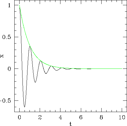
Here's a plot of of an example of such a function $x(t) ~=~ e^{-t}\cos(2\pi t)$

The green line is $A(t) ~=~ e^{-t}$. It is the envelope of the oscillation. Obviously depending on the rate of decay of the amplitude, and the frequency, you'll get a different picture. But qualitatively you'll see an oscillating function whose amplitude decays away to zero. This should describe weak damping. We don't expect this to work too well in molasses. To get a more quantitative understanding we'll have to do some more math.

We'll try sticking $x(t) ~=~ A e^{\lambda t}$ into eqn. 1.60. Here again, $A$ is just a constant. We already differentiated this function before in eqns. 1.24 and 1.25 so we don't have to do it again. So we have

$$m\lambda^2 x + b \lambda x + kx ~=~ 0$$ (1.63)

Canceling the $x$'s

$$m\lambda^2 + b \lambda + k ~=~ 0$$ (1.64)

This is a quadratic equation for $\lambda$. Let's solve it:

$$\lambda ~=~ {-b \pm \sqrt{b^2 -4mk}\over 2m}$$ (1.65)

So we have two possible solutions for $\lambda$! They both solve the equation, and we have to have more information to figure out what to do with them. But for the moment, let's look at this equation more closely.

If the damping, $b$, is large, then the square root is real. However if $b^2 ~<~ 4mk$, then it becomes imaginary.