Let's consider the latter case first. We you get oscillations,
we call this underdamping. In this case  is
a complex number. It's got a real part and an imaginary part.
is
a complex number. It's got a real part and an imaginary part.
The real part is  and we can figure out the imaginary
part by writing
and we can figure out the imaginary
part by writing
 as
as
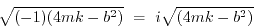 |
(1.66) |
So we can rewrite the solution for as
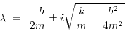 |
(1.67) |
The square root is the magnitude of the imaginary part.
When  , the square root just becomes
  , the
normal frequency of oscillation, so it makes sense to interpret
this as a frequency
, the
normal frequency of oscillation, so it makes sense to interpret
this as a frequency
 |
(1.68) |
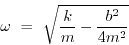
So
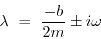 |
(1.69) |
So are solution
 |
(1.70) |
The  means there are two solutions here. This is just like
our earlier use of imaginary numbers to solve the simple
harmonic oscillator. Remember eqn. 1.31. The
two solutions there were shown to be equivalent to the two
solutions in eqn. 1.32. So the same is true
here. The above two solutions are equivalent to
means there are two solutions here. This is just like
our earlier use of imaginary numbers to solve the simple
harmonic oscillator. Remember eqn. 1.31. The
two solutions there were shown to be equivalent to the two
solutions in eqn. 1.32. So the same is true
here. The above two solutions are equivalent to
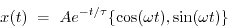
 |
(1.71) |
This is what we guessed above before we plunged into all
this math. You just have an exponential multiplying
a sine wave. But now we know the expression precisely.
The amplitude  decays as
 . What
does this constant mean? If it's zero, there is
no decay at all. If it's big it decays very fast.
. What
does this constant mean? If it's zero, there is
no decay at all. If it's big it decays very fast.
Suppose we start with an amplitude of unity, and want to
know the time  it takes to decay to
 of its
original value. We have
of its
original value. We have
 so at
so at
 we have
 |
(1.72) |
or
 |
(1.73) |
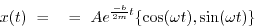
This is often called the the decay time. We can rewrite the
solution in terms of this
 |
(1.74) |
As the damping increases, decreases, that is, it damps faster.
But also note that
as the damping  increases,
  decreases finally hitting
zero. Now we look at what happens past this point.
decreases finally hitting
zero. Now we look at what happens past this point.
josh
2010-01-05